Neural ODE

• Link to paper

• Link to code

Introduction

With motivations from deep learning, neuroscience and mathematics, neural ODE is an attempt to replace layers of neural networks with a continuous-depth model enabled by ODE solvers. The solver parameters are updated using a second ODE solver along with the adjoint method, making it more efficient for both space and time. The model also has a controllable time cost during test and has potential applications in continuous time-series models.

Motivations

Deep Learning Motivation: ResNet

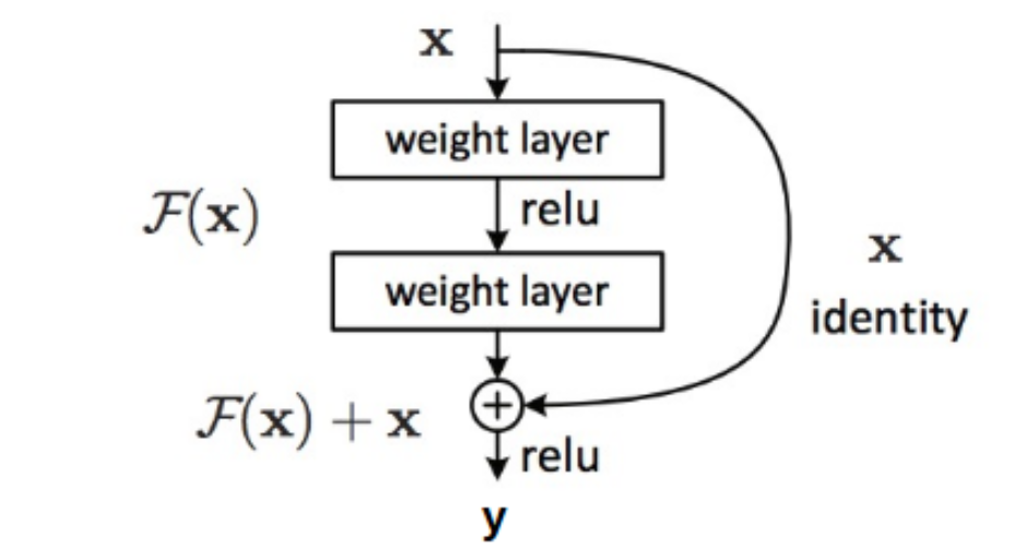
Given a hidden layer that maps $\textbf{x}$ to $\textbf{y}$, a ResNet block enforces $\textbf{y}=F(\textbf{x})+\textbf{x}.$ The motivation is that if you can not do better with more layers, just make $F(\textbf{x})=0$.

Mathematical Motivation: Ordinary Differential Equations (ODE)

Definition (ODE): Equations taking the form of

$$\begin{equation} G(\textbf{x},F(\textbf{x}),F'(\textbf{x}),\cdots,F^{(n)}(\textbf{x}))=0 \end{equation}$$

ODEs can be helpful for describing a continuous time system. Consider $\textbf{z}:t\mapsto\textbf{z}(t), \mathbb{R}\rightarrow\mathbb{R}^{n}$

$$\begin{equation} G(t,\textbf{z}(t), \textbf{z}'(t))=0\Longleftrightarrow \textbf{z}'(t)=f(\textbf{z}(t), t) \end{equation}$$

In ODE, we are usually interested in solving an initial value problem:

Given

$$\begin{cases} \textbf{z}(0)\\ \textbf{z}'(t)=f(\textbf{z}(t), t) \end{cases}$$

we want to know $\textbf{z}(t)=\textbf{z}(0)+\int_{0}^{t}\textbf{z}'(t).$

When it is difficult or impossible to solve $\textbf{z}(t)$, we can numerically approximate it at points of interest. This is what people working in numerical differential equations/computational mathematics are doing.

The most basic method is Euler's method: $\textbf{z}(t_{0}+h)\approx\textbf{z}(t_{0})+h\textbf{z}'(t_0)$

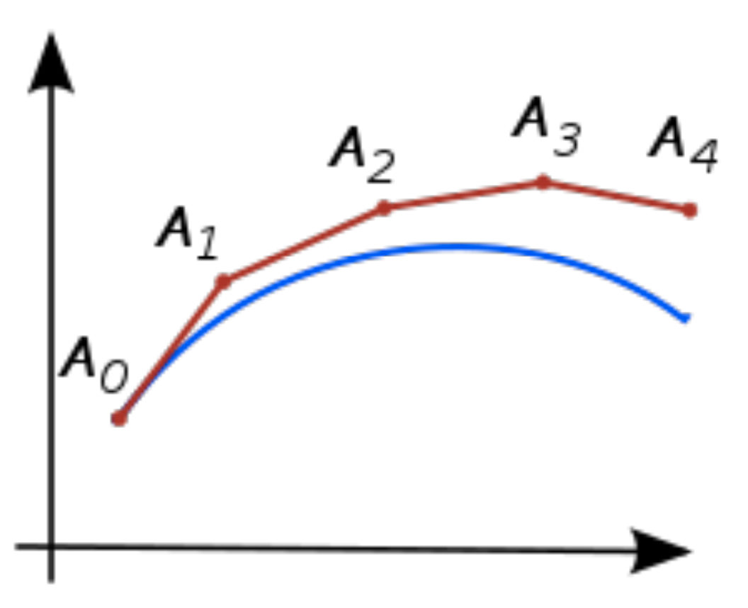
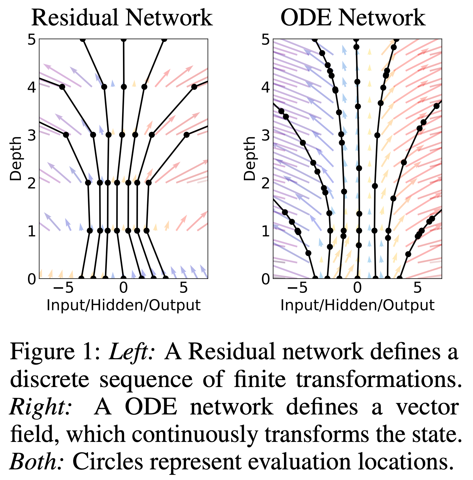
Comparing with ResNet: $\textbf{y}=\textbf{x}+F(\textbf{x})$, we can view each Residual layer as performing $\textbf{z}(\textbf{x})\mapsto\textbf{z}(\textbf{x}+1)$, the final output is just $\textbf{z}(T)$.

But it seems that $h$ can take any real value, then can we have infinite number of layers?

Yes!

Neuroscience Motivation

Real brains are continuous time systems, hence early neural network research takes continuous time systems as a starting point.

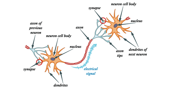
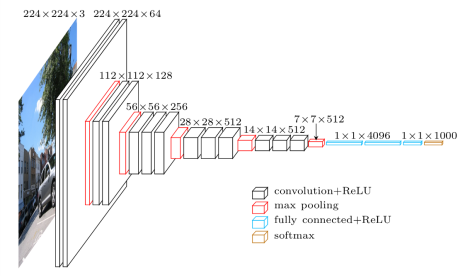
Artificial Neural Networks today model brain with discretization.

Proposal

We can modify ResNet to make it more ODE alike with a continuous time system!

def f(z, t, theta):
    return nnet(z, theta[t])

def resnet(z, theta):
    for t in [1:T]:
        z = z + f(z, t, theta)
    return z

$$\begin{equation} \Downarrow \end{equation}$$

def f(z, t, theta):
    return nnet([z, t], theta)

def resnet(z, theta):
    for t in [1:T]:
        z = z + f(z, t, theta)
    return z

We can replace resnet with an ODE solver, which approximates $\int_{t_{0}}^{t_1}f(\textbf{z}(t), t, \theta)dt$.

BP through ODE Solvers

We want to optimize

$$\begin{equation} L(\text{ODESolve}(\textbf{z}(t_0), f, t_0, t_1, \theta)) \end{equation}$$

by changing its parameters $\textbf{z}(t_0), t_0,t_1,\theta$.

Direct BP is slow, with extra numerical error and memory cost.

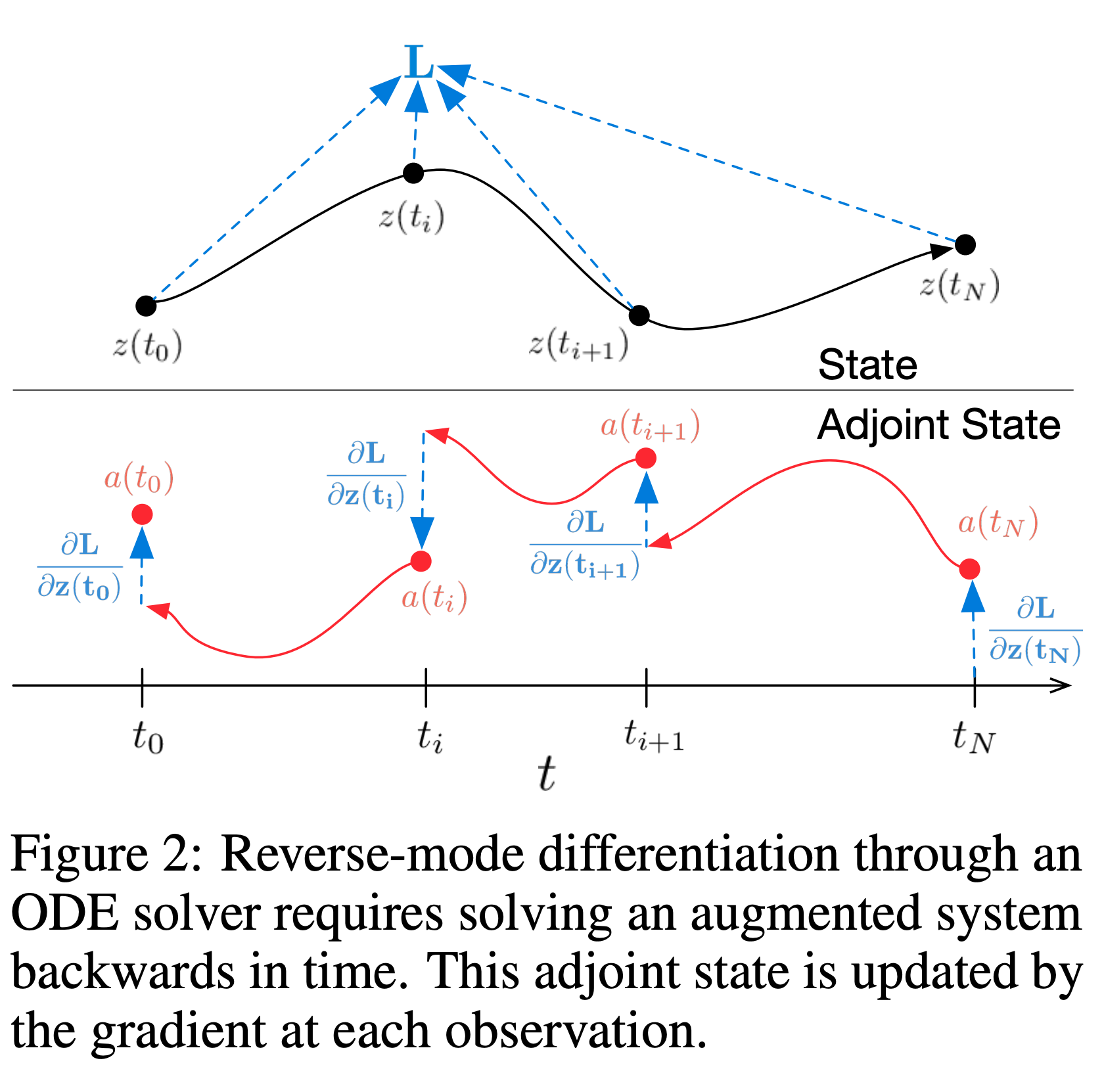
The authors compute gradients using the adjoint method, which directly approximates the gradient, rather than differentiating the approximation. Proof can be found here.

This approach computes gradients by solving a second, augmented ODE backwards in time, and is applicable to all ODE solvers.

The key results from the proof are as follows:

• Let $\textbf{a}(t)=\frac{\partial L}{\partial \textbf{z}(t)}$

• $\frac{d\textbf{a}(t)}{dt}=-\textbf{a}(t)^{T}\frac{\partial f(\textbf{z}(t), t, \theta)}{\partial\textbf{z}}$

• $\frac{dL}{d\theta}=\int_{t_1}^{t_0}\textbf{a}(t)^{T}\frac{\partial f(\textbf{z}(t),t,\theta)}{\partial \theta}dt$

When the loss depends on intermediate states, the reverse-mode derivative must be broken into a sequence of separate solves.

Experiments in Supervised Learning

The authors compared the performance of a small residual network which downsamples the input twice then applies 6 residual blocks, which are replaced by an ODESolve module in the ODE-Net variant. They also tested a network which directly BP through a Runge-Kutta integrator (a numerical method for iteratively solving an nonlinear ODE), referred to as RK-Net.

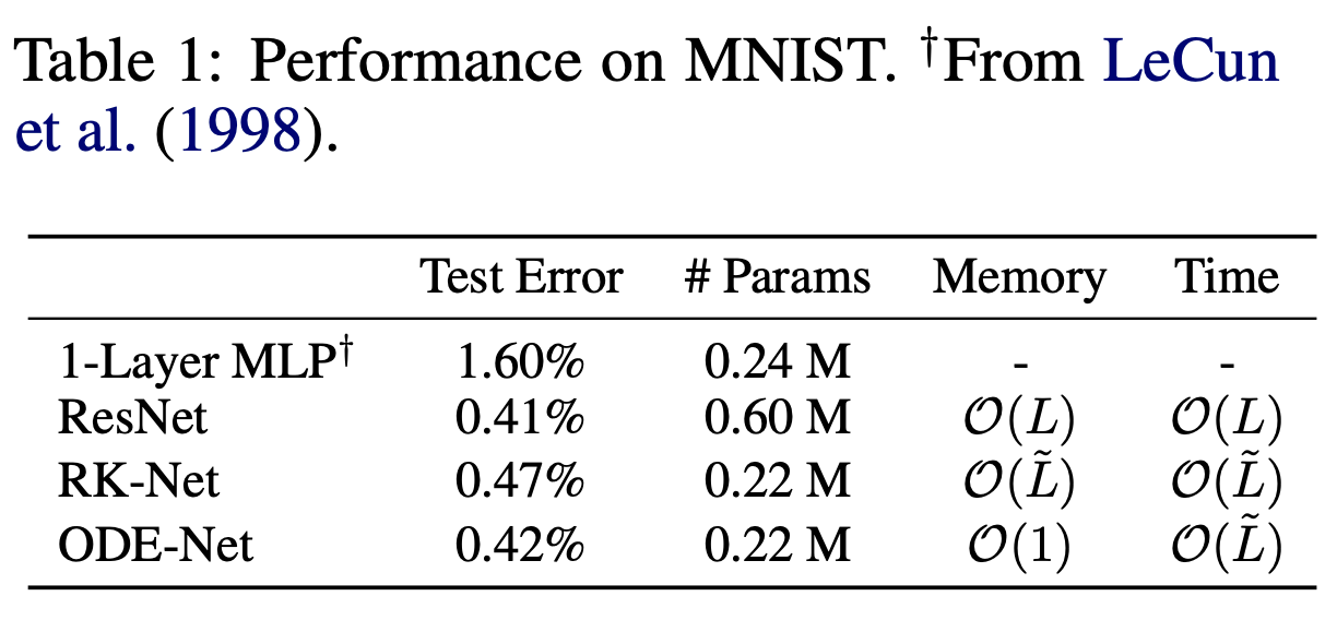
In the figure above, $L$ denotes the number of layers in the ResNet and $\tilde{L}$ denotes the number of function evaluations that the ODE solver requests in a single forward pass, which can be interpreted as an implicit number of layers.

For reference, a neural net with a single hidden layer of $300$ units has around the same number of parameters as the ODE-Net and RK-Net architecture.

One advantage of using ODE solvers is that many of them approximately ensure that the output is within a given tolerance of the true solution.

The authors verify that error can indeed be controlled in figure 3a. They also show that tunning the tolerance gives us a trade-off between accuracy and computational cost with figure 3b.

Figure 3c shows that the number of evaluations in the backward time is roughly half of the forward pass. This suggests that the adjoint sensitivity method is not only more memory efficient, but also more computationally efficient than direct BP.

Note that it is not clear how to define the "depth" of an ODE solution. A related quantity is the number of evaluations of the hidden state dynamics required, a detail delegated to the ODE solver and dependent on the initial state or input. In figure 3d, the authors show that the number of function evaluations increases throughout training, presumably adapting to increasing complexity of the model. Note that Duvenaud mentioned that their model in the end can be 2-4x slower than ResNet.

Continuous Normalizing Flows

The discretized equation

$$\begin{equation} \textbf{h}_{t+1}=\textbf{h}_{t}+f(\textbf{h}_{t}, \theta_t) \end{equation}$$

also appears in normalizing flows and the NICE framework. These methods use the change of variables theorem to compute exact changes in probability if samples are transformed through a bijective function $f$:

$$\begin{equation} \textbf{z}_1=f(\textbf{z}_0) \Longrightarrow \log p(\textbf{z}_1)=\log p(\textbf{z}_0)-\log\left|\det\frac{\partial f}{\partial \textbf{z}_0}\right| \end{equation}$$

Generally, the main bottleneck to using the change of variables formula is computing of the determinant of the Jacobian $\frac{\partial f}{\partial \textbf{z}}$, which has a cubic cost in either the dimension of $\textbf{z}$, or the number of hidden units.

Surprisingly, moving from a discrete set of layers to a continuous transformation simplifies the computation of the change in normalizing constant.

Theorem (Instantaneous Change of Variables). Let $\textbf{z}(t)$ be a finite continuous random variable with probability $p(\textbf{z}(t))$ dependent on time. Let $\frac{d\textbf{z}}{dt}=f(\textbf{z}(t), t)$ be a differential equation describing a continuous-in-time transformation of $\textbf{z}(t)$. Assuming that $f$ is uniformly Lipschitz continuous ($\exists$ an universal Lipschitz constant) in $\textbf{z}$ and continuous in $t$, then the change in log probability also follows a differential equation,

$$\begin{equation} \frac{\partial \log p(\textbf{z}(t))}{\partial t}=-\text{tr}\left(\frac{df}{d\textbf{z}(t)}\right). \end{equation}$$

Proof. Let $\textbf{z}(t+\epsilon)=T_{\epsilon}(\textbf{z}(t))$. We assume that $f$ is Lipschitz continuous in $\textbf{z}(t)$ and continuous in $t$, so every initial value problem has a unique solution by Picard's existence theorem. We also assume $\textbf{z}(t)$ is bounded. These conditions imply that $f, T_{\epsilon}$ and $\frac{\partial}{\partial \textbf{z}}T_{\epsilon}$ are all bounded.

$$\begin{align} \frac{\partial\log p(\textbf{z}(t))}{\partial t}&=\lim_{\epsilon\rightarrow 0^{+}}\frac{\log p(\textbf{z}(t))-\log\left|\det\frac{\partial}{\partial\textbf{z}}T_{\epsilon}(\textbf{z}(t))\right|-\log p(\textbf{z}(t))}{\epsilon}\\ &=-\lim_{\epsilon\rightarrow 0^{+}}\frac{\log\left|\det\frac{\partial}{\partial\textbf{z}}T_{\epsilon}(\textbf{z}(t))\right|}{\epsilon}\\ &=-\lim_{\epsilon\rightarrow 0^{+}}\frac{\frac{\partial}{\partial\epsilon}\left|\det\frac{\partial}{\partial\textbf{z}}T_{\epsilon}(\textbf{z}(t))\right|}{\left|\det\frac{\partial}{\partial\textbf{z}}T_{\epsilon}(\textbf{z}(t))\right|} \text{ (by L'Hopital's rule)}\\ &=-\left(\lim_{\epsilon\rightarrow 0^{+}}\frac{\partial}{\partial\epsilon}\left|\det\frac{\partial}{\partial\textbf{z}}T_{\epsilon}(\textbf{z}(t))\right|\right)\left(\lim_{\epsilon\rightarrow 0^{+}}\frac{1}{|\det\frac{\partial}{\partial\textbf{z}}T_{\epsilon}(\textbf{z}(t))|}\right)\\ &=-\lim_{\epsilon\rightarrow 0^{+}}\frac{\partial}{\partial\epsilon}\left|\det\frac{\partial}{\partial\textbf{z}}T_{\epsilon}(\textbf{z}(t))\right| \end{align}$$

The derivative of the determinant can be expressed using Jacobi's formula, which gives

$$\begin{align} \frac{\partial \log p(\textbf{z}(t))}{\partial t} &= -\lim_{\epsilon\rightarrow 0^{+}}\text{tr}\left(\text{adj}\left(\frac{\partial}{\partial\textbf{z}}T_{\epsilon}(\textbf{z}(t))\right)\frac{\partial}{\partial\epsilon}\frac{\partial}{\partial\textbf{z}}T_{\epsilon}(\textbf{z}(t))\right)\\ &=-\text{tr}\left(\left(\lim_{\epsilon\rightarrow 0^{+}}\text{adj}\left(\frac{\partial}{\partial\textbf{z}}T_{\epsilon}(\textbf{z}(t))\right)\right)\left(\lim_{\epsilon\rightarrow 0^{+}}\frac{\partial}{\partial \epsilon}\frac{\partial}{\partial\textbf{z}}T_{\epsilon}(\textbf{z}(t))\right)\right)\\ &=-\text{tr}\left(\lim_{\epsilon\rightarrow 0^{+}}\frac{\partial}{\partial \epsilon}\frac{\partial}{\partial\textbf{z}}T_{\epsilon}(\textbf{z}(t))\right) \end{align}$$

By expanding the Taylor series around $\textbf{z}(t)$, the equation above equals to

$$\begin{equation} -\text{tr}\left(\frac{\partial}{\partial\textbf{z}}f(\textbf{z}(t), t)\right) \end{equation}$$

The proof has been finished now.

Trace is a much cheaper operation, which has a square cost in either the dimension of $\textbf{z}$, or the number of hidden units.

Generative latent function time-series model

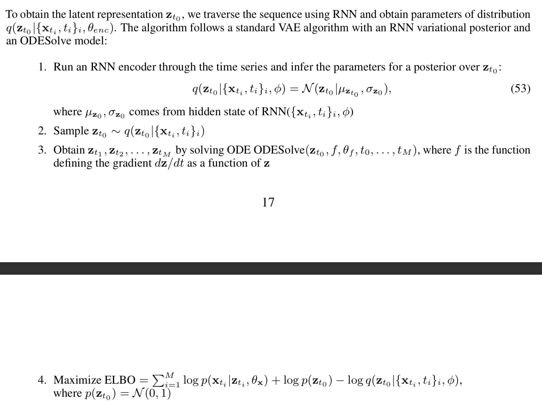
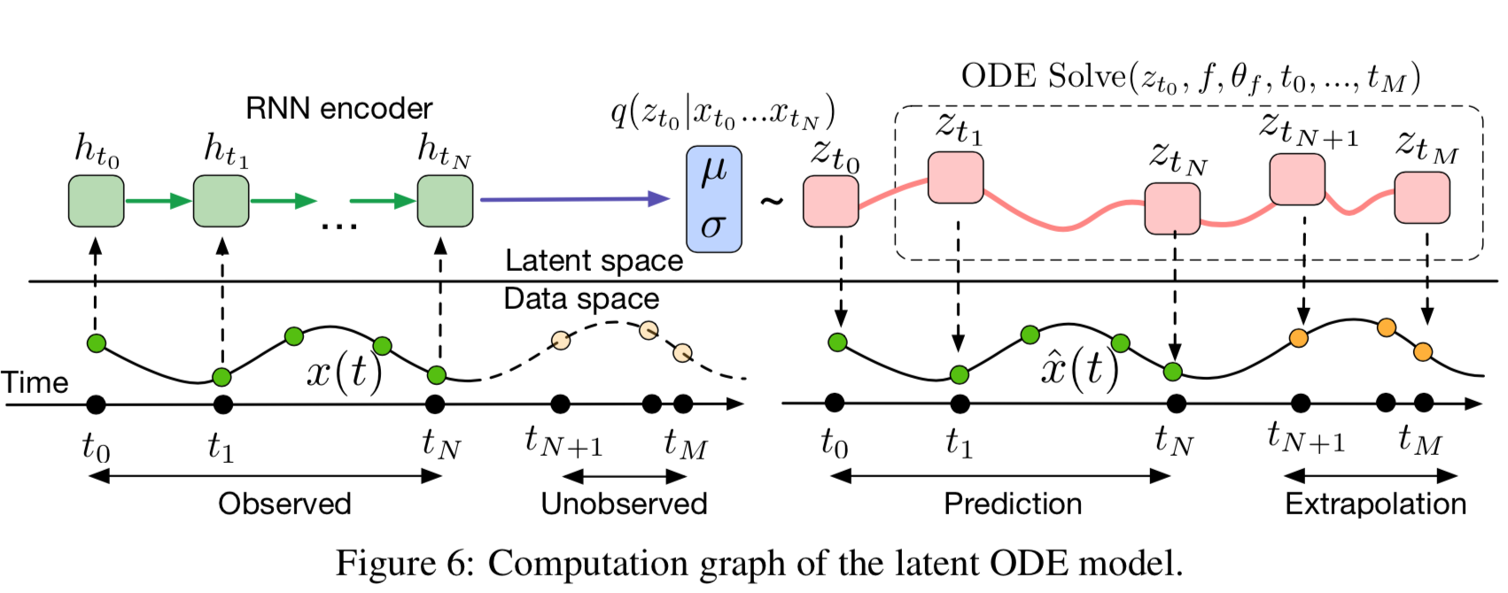
The authors present a continuous-time generative approach to modeling time series. Their model represents each time series by a latent trajectory. Each trajectory is determined from a local initial state $\textbf{z}_{t_0}$, and a global set of latent dynamics shared across all time series. Given observation times $t_0, t_1,\cdots, t_N$ and an initial state $\textbf{z}_{t_0}$, an ODE solver produces $\textbf{z}_{t_1},\cdots, \textbf{z}_{t_N}$, which describe the latent state at each observation. They define this generative model fromally through a sampling procedure:

$$\begin{align} \textbf{z}_{t_0}&\sim p(\textbf{z}_{t_0})\\ \textbf{z}_{t_1},\textbf{z}_{t_2},\cdots,\textbf{z}_{t_N} &= \text{ODESolve}(\textbf{z}_{t_0},f,\theta_f,t_0,\cdots, t_N)\\ \textbf{x}_{t_i}&\sim p(\textbf{x}|\textbf{z}_{t_i},\theta_{\textbf{x}}) \end{align}$$

Function $f$ is a time-invariant function that takes the value $\textbf{z}$ at the current time step and outputs the gradient: $\frac{\partial\textbf{z}(t)}{\partial t}=f(\textbf{z}(t),\theta_f)$. The function is parametrized using an NN. Because $f$ is time-invariant, given any latent space $\textbf{z}(t)$, the entire trajectory is uniquely defined. Extrapolating this latent trajectory lets us make predictions arbitrarily far forwards or backwards in time.

Benefits

Benefits of differentiable ODE solvers include: 1. Memory efficiency: no intermediate variabels stored for chain rule, hence constant memory cost 2. Adaptive computation: the choice of ODE solver is orthogonal, different ODE solvers can be used for a same model. There are theories for ODE solvers with more than 120 years of development. Modern ODE solvers allow a controllable trade off between time cost and precission during test time. 3. Parameter sharing across layers 4. Easier computation for changing variables 5. Continuous time-series models