How Powerful are Graph Neural Networks?

Motivation

The design of new GNNs is mostly based on empirical intuition, heuristics, and experimental trial-and-error. There is little understanding of the properties and limitations of GNNs, and formal analysis of GNNs' representational capacity is limited.

Contributions and Conclusions

1. GNNs are at most as powerful as the WL test in distinguishing graph structures.

2. Established conditions on the neighbor aggregation and graph pooling functions under which the resulting GNN is as powerful as the WL test.

3. Identified graph structures that cannot be distinguished by popular GNN variants, such as GCN and GraphSAGE and characterized the kinds of graph structures such GNN-based models can capture.

4. Developed a simple neural architecture, Graph Isomorphism Network (GIN) and showed that its discriminative/representational power is equal to the power of the WL test.

Preliminaries

A layer of a GNN can be formulated as

$$\begin{align} a_{v}^{(k)}&=\text{AGGREGATE}^{(k)}\left(\{h_{u}^{(k-1)}:u\in\mathcal{N}(v)\}\right)\\ h_{v}^{(k)}&=\text{COMBINE}^{(k)}(h_{v}^{(k-1)}, a_{v}^{(k)}), \end{align}$$

where $h_{v}^{(k)}$ is the feature vector of the node $v$ at the $k$-th iteration/layer, $h_{v}^{(0)}$ is set to be the original node features $X_v$, $\mathcal{N}(v)$ is the set of one-hop neighbors of $v$. The choice of $\text{AGGREGATE}^{(k)}(\cdot)$ and $\text{COMBINE}^{(k)}(\cdot)$ in GNNs is crucial.

For node classification, $h_{v}^{(K)}$ of the final iteration is used for prediction. For graph classification, a $\text{READOUT}$ function is used on the features of all nodes in a graph. Some common choices are simply to take the average or summation. A frequently desired property is permutation invariance.

Weisfeiler-Lehman (WL) test

The graph isomorphism problem asks whether two graphs are topologically equivalent, i.e. you can obtain one graph from the other by relabeling the nodes. This problem is known to be NP. Despite some corner cases, the WL test of graph isomorphism is an effective and computationally efficient test that distinguishes a broad class of graphs.

The 1-d form of WL test, "naive vertex refinement" is analogous to neighborhood aggregation in GNNs. The WL test is based on node attributes. If the graph has no node attributes, then simply assign all of them some constant value. Iteratively, this test updates node features with

$$\begin{equation} h_v \leftarrow \text{hash}\left(\sum_{u\in\mathcal{N}(v)}h_u\right), \end{equation}$$

where the node features are scalars and $\text{hash}(\cdot)$ is ideally an injective hash function. The test repeats for a fixed number of steps or until convergence. The algorithm decides that two graphs are different if at some iteration their node labels are different.

WL test is not guaranteed to work for all graphs. In particular, it fails for graphs with a high degree of symmetry, e.g. chains, complete graphs, tori and stars.

Weisfeiler-Lehman Graph Kernels proposed the WL subtree kernel that measures the similarity between graphs. The kernel uses the counts of node labels at different iterations of the WL test as the feature vector of a graph and has the same discriminative power as the WL testIntuitively, a node's label at the $k$-th iteration of WL test represents a subtree structure of height $k$ rooted at the node:

Aggregation as a Function Applied to Multisets

The authors assume that the node features are from a countable universe. Then, feature vectors of a set of neighboring nodes form a multiset: the same element can appear multiple times since different nodes can have identical feature vectors.

Intuitively, the most powerful GNN should map two nodes to the same embedding only when their neighborhoods are the same multiset, i.e. the mapping is injective. Thus they abstract a GNN's aggregation as a class of functions over multisets that its neural network can represent, and analyze whether they are able to represent injective multiset functions.

Building Powerful Graph Neural Networks

The authors aim to solve the following problem: when do graph neural networks have the same discriminative capacity as WL test? In other words, we want a GNN to map different graphs onto different embeddings iff the WL test decides they are non-isomorphic. The conclusions are: 1. If $G_1$ and $G_2$ do not have the same embedding with a GNN, they will be decided non-isomorphic with the WL test. 2. The GNN will have the same discriminative power as the WL test when $\text{AGGREGATE}, \text{COMBINE}, \text{READOUT}$ are all injective on multisets.

Graph Isomorphism Network

The authors developed a graph neural network that generalizes WL test, termed as Graph Isomorphism Network (GIN).

Aggregation and Concatenation

The authors prove that choosing

$$h_{v}^{(k)} = \text{MLP}^{(k)}\left((1+\epsilon^{(k)})\cdot h_{v}^{(k-1)}+\sum_{u\in\mathcal{N}(v)}h_{u}^{(k-1)}\right)$$

gives the integration of an injective $\text{AGGREGATE}$ and $\text{COMBINE}$ functions.

First, they show that the following proposition holds:

Assume $\mathcal{X}$ is countable. There exists a function $f:\mathcal{X}\rightarrow\mathbb{R}^{n}$ so that for infinitely many choices of $\epsilon$, including all irrational numbers, $h(c, X)=(1+\epsilon)\cdot f(c)+\sum_{x\in X}f(x)$ is unique for each pair $(c, X)$ where $c\in \mathcal{X}$ and $X\subset\mathcal{X}$ is a finite multiset. Moreover any function $g$ over such pairs can be decomposed as $g(c, X)=\phi\left((1+\epsilon)\cdot f(c)+\sum_{x\in X}f(x)\right)$ for some function $\phi$.

If the proposition holds, then the update rule follows by approximating $\phi\circ f$ with an MLP. $\epsilon$ can be either a learnable parameter or a fixed scalar.

"""
Personal comment:

If you have node attributes that are too close to each other, I think sum 
aggregation will still fail without transforming node features for 
polarization first.
"""

Before we prove the proposition, let's first present a lemma and its proof.

Lemma: Assume $\mathcal{X}$ is countable. There exists $f:\mathcal{X}\rightarrow\mathbb{R}^{n}$ so that $h(X)=\sum_{x\in X}f(x)$ is unique for each multiset $X\subset\mathcal{X}$. Moreover, any multiset function $g$ can be decomposed as $g(X)=\phi\left(\sum_{x\in X}f(x)\right)$ for some function $\phi$.

Proof: Since $\mathcal{X}$ is countable, there exists $Z:\mathcal{X}\rightarrow\mathbb{N}$. Since the multisets $X$ are finite, $\exists N\in\mathbb{N}$ so that $|X|< N$ for all $X$. Then an example of such $f$ is $f(x)=N^{-Z(x)}$. This $f$ can be viewed as a more compressed form of an one-hot vector or $N$-digit presentation. Thus $h(X)=\sum_{x\in X}f(x)$ is an injective function of multisets. $\phi(\sum_{x\in X}f(x))$ is permutation invariant so it is a well-defined multiset function. For any multiset function $g$, we can construct such $\phi$ by letting $\phi(\sum_{x\in X}f(x))=g(X)$.

Proof for the proposition: Consider $h(c, X)$ defined in the proposition with $\epsilon$ being an irrational number and $f$ defined as above. We will prove that whenever $(c_1, X_1)\neq (c_2, X_2), c_1, c_2\in\mathcal{X}, X_1,X_2\subset\mathcal{X}$, $h(c_1, X_1)\neq h(c_2,X_2)$. We will discuss two separate cases: 1) $c_1=c_2, X_1\neq X_2$; 2) $c_1\neq c_2$. The first case follows directly from the previous proof. For the second case we can prove by contradiction. Assume $h(c_1,X_1)=h(c_2, X_2)$, we have

$$\epsilon(f(c_1)-f(c_2)) = \left(f(c_2)+\sum_{x\in X_2}f(x)\right)-\left(f(c_1)+\sum_{x\in X}f(x)\right).$$

Since the left handside is irrational and the right handside is rational, this cannot be true.

Readout

The number of rounds for message passing/graph convolution can have a huge effect on the updated features. To address this issue, the authors simply consider the node features of all levels:

$$h_{G} = \text{CONCAT}(\text{READOUT}\left(\{h_{v}^{(k)}|v\in G\}\right)|k=0,1,\cdots, K)$$

Study on GNNs

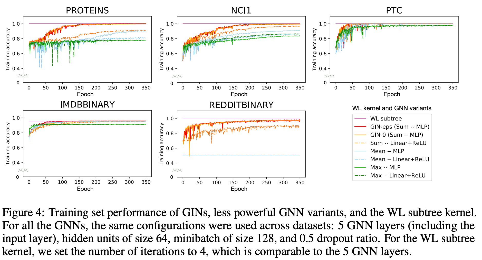
To understand better the popular GNNs, the authors perform an ablation study on aggregation: (1) $1$-layer perceptrons instead of MLPs and (2) mean or max-pooling instead of the sum. They show that while GCN can perform well on node classification, GNNs like GCN and GraphSAGE are less powerful than WL test.

1-Layer Perceptrons are not Sufficient

The authors prove that there exists multisets $X_1\neq X_2$ so that for any linear mapping $W$, $\sum_{x\in X_1}\text{ReLU}(Wx)=\sum_{x\in X_2}\text{ReLU}(Wx)$.

Counter Example: Consider $X_{1}\neq X_{2}$ consisting of scalars that are of the same sign (either all positive or all nonnegative) and $\sum_{x\in X_1}x=\sum_{x\in X_2}x$. Then by nonlinearity we have $\text{ReLU}(\sum_{x\in X_1}Wx)=\text{ReLU}(\sum_{x\in X_2}Wx)$. Hence the aggregator is not an injective function on multisets.

Note that the original GCN does not have a bias term and with a bias term things might be better. Meanwhile, we need at least one hidden layer for Universal Approximation Theorem to hold. The authors claim that this may result in an underfitting model that cannot well capture the structural information.

Structures that Confuse Mean and Max-Pooling

Two common aggregation methods are mean pooling and max pooling as they are invariant under node permutation. However these methods can fail on some regular graphs particularly when the multiplicity/number of occurrence/counting of node features also matters.

In the toy binary graph classification example I tried, if you do not give node degrees as node features at the beginning, you will not be able to even distinguish cycles from stars.

"""
Personal comment:

As mentioned before, the sum aggregation can still fail, in which case we
may need some node embedding module as in DGMG.

When node features are diverse and rarely repeat, mean aggregation may still
be enough and the authors attribute the success of GCN to this case.
"""

Experiments

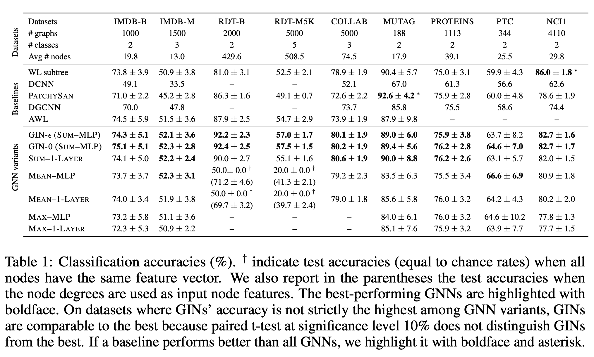
Graph classification is performed on 9 benchmarks with the dataset statistics and performance summarized in the table below:

Some clarifications: 1. For their model GIN, they used two variants, GIN-$\epsilon$ learns $\epsilon$ via gradient descent in $h_{v}^{(k)} = \text{MLP}^{(k)}\left((1+\epsilon^{(k)})\cdot h_{v}^{(k-1)}+\sum_{u\in\mathcal{N}(v)}h_{u}^{(k-1)}\right)$, GIN-$0$ simply fixes $\epsilon=0$. While GIN-$0$ consistently outperforms GIN-$\epsilon$, there exists certain graphs that GIN-$\epsilon$ and the WL test can distinguish but GIN-$0$ cannot. 2. For REDDIT-BINARY, REDDIT-MULTI5K and COLLAB, they did not run experiments for max-pooling due to GPU memory constraints. 3. The other GNN variants correspond to replace the corresponding aggregator or readout in GIN. I think it will still be nice to test on the standard GNNs as there still exists some slight difference from the formulation of authors. 4. For baselines, DCNN stands for Diffusion-convolutional neural networks; DGCNN stands for Deep Graph CNN; and AWL stands for Anonymous Walk Embeddings. 5. t-test is a statistical hypothesis test and is most commonly applied when the test statistics would follow a normal distribution. I personally do not believe much the p-value staff.

Future Work

1. Analyze more complicated aggregation like the one used in GAT and the LSTM pooling in GraphSAGE.

2. Go beyond hashing and measure how well the similarity of nodes and graphs are preserved with the embeddings.