Layerwise Adaptive Sampling

tags: GCN, sampling, NeuralPS2018

Adaptive Sampling Towards Fast Graph Representation Learning

Multiple vertices may have some common neighbors so neighbor sampling can result in repeated samples. We can avoid the over-expansion and accelerate the training of GCN by controlling the size of the sampled neighborhoods in each layer.

The core of the method is to define an appropriate sampler for the layer-wise sampling. A common objective to design the sampler is to minimize the resulting variance. Unfortunately, the optimal sampler to minimize the variance is uncomputable due to the inconsistency between the top-down sampling and the bottom-up propagation in our network. To tackle this issue a parametrized sampler is used and the resulting variance, being a loss term, can be directly optimized with BP.

The authors also propose to include skip connection for message passing so that 2nd order proximity

To sum up, the contributions include:

• Overexpansion of neighborhood $\Rightarrow$ Layer-wise neighbor sampling

• Uncomputable optimal sampler $\Rightarrow$ Feature based parametrized sampler + directly optimizing variance in the objective

• Preserving 2nd order proximity $\Rightarrow$ Skip connection for message passing

Related Work

• Spectral: defines the convolution operation in Fourier domain

  • Spectral networks and locally connected networks on graphs: defines the convolution operation in Fourier domain

  • Deep convolutional networks on graph-structured data: enables localized filtering by applying efficient spectral filters

  • Convolutional neural networks on graphs with fast localized spectral filtering: employs Chebyshev expansion of the graph Laplacian to avoid the eigendecomposition

  • GCN: simplify previous methods with first-order expansion and re-parameterization trick

• Non-spectral: define convolution on graph by using the spatial connections directly

  • Convolutional neural networks on graphs for learning molecular fingerprints: learns a weight matrix for each node degree

  • Diffusion-convolutional neural networks: defines multiple-hop neighborhoods by using the power series of a transition matrix

  • Learning convolutional neural networks for graphs: extracts normalized neighborhoods that contain a fixed number of nodes

• Leap of model capacity: implicitly weight node importance of a neighborhood

  • Geometric deep learning on graphs and manifolds using mixture model cnns: build ConvNet on graphs using the patch operation

  • GAT: compute the hidden representations of each node on graph by attending over its neighbors following a self-attention strategy

Method Formulation

Monte Carlo GCN

In GCN, the update rule for node features is

$$h_{v}^{(l+1)} = \sigma\left(\sum_{u\in\mathcal{N}(v)\bigcup\{v\}}\hat{A}(u,v)h_{u}^{(l)}W^{(l)}\right),$$

where

$$\hat{A}(u, v)=\left(\hat{D}^{-\frac{1}{2}}\hat{A}\hat{D}^{-\frac{1}{2}}\right)_{u, v}.$$

We can reformulate the rule above with expectation:

$$h_{v}^{(l+1)} = \sigma\left(N(v)\mathbb{E}_{u\sim p(u|v)}[h_u^{(l)}]W^{(l)}\right),$$

where

$$N(v)=\sum_{u\in\mathcal{N}(v)\bigcup\{v\}}\hat{A}(u, v), p(u|v)=\frac{\hat{A}(u,v)}{N(v)}.$$

The term $\mathbb{E}_{u\sim p(u|v)}[h_u^{(l)}]$ may be approximated with Monte Carlo sampling:

$$\frac{1}{n}\sum_{i=1}^{n}h_{u_i}^{(l)},$$

with $u_1,\cdots,u_n$ sampled with $p(u|v)$.

Layer-wise sampling

The layer-wise sampling can be incorporated with importance sampling. Assume $q(u|v_1,\cdots, v_m)$ is a conditional layer-wise sampling distribution, which we will introduce later. The original update rule is equivalent to

$$h_v^{(l+1)}=\sigma\left(N(v)\mathbb{E}_{u\sim q(u|v_1,\cdots,v_m)}\left[\frac{p(u|v)}{q(u|v_1,\cdots,v_m)}h_u^{(l)}\right]W^{(l)}\right),$$

where $v\in\{v_1,\cdots,v_m\}$. We can also perform Monte Carlo sampling as above.

Opposed to the node-wise Monte Carlo method where the nodes are sampled independently for each $v_i$, the layer-wise sampling is performed only once for $v_1,\cdots,v_m$. As a result, the total number of sampling nodes only grows linearly with the network depth if we fix the sampling size n.

Variance reduction

For simplicity we abbreviate $q(u|v_1,\cdots,v_m)$ as $q(u)$. For a good choice of $q(u)$, we seek to reduce the induced variance of $\hat{\mu}_{q}(v_j)=\frac{1}{n}\sum_{i=1}^{n}\frac{p(u_i|v_j)}{q(u_i)}h_{u_i}^{(l)}$, $v_j\in\{v_1,\cdots,v_m\}$, $u_i$'s are sampled from $q(u)$.

Note that there is a small problem with the original argument of the authors where they treat $h_{u_i}^{(l)}$ as a scalar rather than a vector. The argumentation there was more for some motivation.

If $h_{u_i}^{(l)}$ is a scalar, then as mentioned in page 6, Chapter 9 Importance Sampling, Monte Carlo theory, methods and examples, the variance is

$$\frac{1}{n}\mathbb{E}_{q}\left[\frac{(h_{u_i}^{(l)}p(u_i|v_j)-q(u_i)\mathbb{E}_p[h_{u_i}^{(l)}])^2}{q(u_i)^2}\right]$$

and the optimal $q$ in terms of variance is given by

$$\frac{p(u_i|v_j)|h_{u_i}^{(l)}|}{\mathbb{E}_{p}[|h_{u_i}^{(l)}|]}.$$

For both reasons that: 1. $h_{u_i}^{(l)}$ is a vector and we want a scalar 2. Even the above holds, $\mathbb{E}_{p}[|h_{u_i}^{(l)}|]$ cannot be evaluated efficiently.

The authors use a linear layer $g(x(u_i))=W_gx(u_i)$ to replace $h_{u_i}^{(l)}$ in the eqution above, where $W_g\in\mathbb{R}^{1\times D}$. $x(u_i)$ is the node feature. We can then perform a Monte Carlo estimation

$$\frac{p(u_i|v_j)|g(x(u_j))|}{\sum_{i=1}^{N}p(u_i|v_j)|g(x(u_i))|}.$$

To make the estimation independent of $v_j$ for the purpose of layerwise sampling, we can do

$$q(u_i)=\frac{\sum_{j=1}^{m}p(u_i|v_j)|g(x(u_j))|}{\sum_{i=1}^{N}\sum_{j=1}^{m}p(u_i|v_j)|g(x(u_i))|}.$$

To make the variance reduction process adaptive, we can directly add the estimated variance to the objective function:

$$\frac{1}{n^2}\sum_{i=1}^{n}\frac{\left(p(u_i|v_j)g(x(u_i))-\hat{\mu}_q(v_j)q(u_i)\right)^2}{q^2(u_i)},$$

where $u_1,\cdots,u_n$ are sampled from $q$.

Skip Connections

For the nodes of the $(l+1)$ layer, we can add direct connections between them and the nodes in the $(l-1)$ layer for feature update.

$$h_{skip}^{(l+1)}(v_i) = \sum_{j=1}^{n}\hat{a}_{skip}(v_i, s_j)h_{s_j}^{(l-1)}W_{skip}^{(l-1)},$$

where:

• $\{s_j\}_{j=1}^{n}$ are nodes sampled in the $(l-1)$-th layer.

• $\hat{a}_{skip}(v_i,s_j)$ is approximated by $\sum_{k=1}^{n}\hat{a}(v_i, u_k)\hat{a}(u_k, s_j)$ where $u_1,\cdots,u_k$ are nodes sampled in the $l$-th layer.

• $W_{skip}^{(l-1)}=W^{(l-1)}W^{(l)}$, where $W^{(l)}$ and $W^{(l-1)}$ are the filters of the $l$-th and $(l-1)$-th layers

The final update is then

$$h_{v}^{(l+1)} = \sigma\left(h_{skip}^{(l+1)}(v)+\sum_{u\in\mathcal{N}(v)\bigcup\{v\}}\hat{A}(u,v)h_{u}^{(l)}W^{(l)}\right).$$

Attention

In GAT, $\hat{A}(u,v)$ is replaced by $\text{SoftMax}(\text{LeakyReLU}(W_{1}h^{(l)}(v_i), W_{2}h^{(l)}(u_j)))$, the dependence on $h^{(l)}(v_i), h^{(l)}(u_j)$ makes it intractable for the method proposed as the sampling of nodes in the $l$ th layer depends on the nodes in the $l+1$ th layer. The author proposed to use

$$\frac{1}{n}\text{ReLU}(W_{1}(g x(v_i)) + W_{2}g(x(u_j)))$$

instead, where $W_{1}$ and $W_2$ and $x(v_i), x(u_j)$ are the node features.

Experiments

• Categorizing academic papers in the citation network datasets -- Cora ($O(10^3)$ nodes), Citeseer ($O(10^3)$ nodes) and Pubmed ($O(10^4)$ nodes)

• Predicting which community different posts belong to in Reddit ($O(10^5)$ nodes)

The sampling framework is inductive (separates out test data from training) rather than transductive (all vertices are included). In test time, the authors do not use sampling.

The experiments are conducted with random seeds over $20$ trials with mean and standard variances recorded.

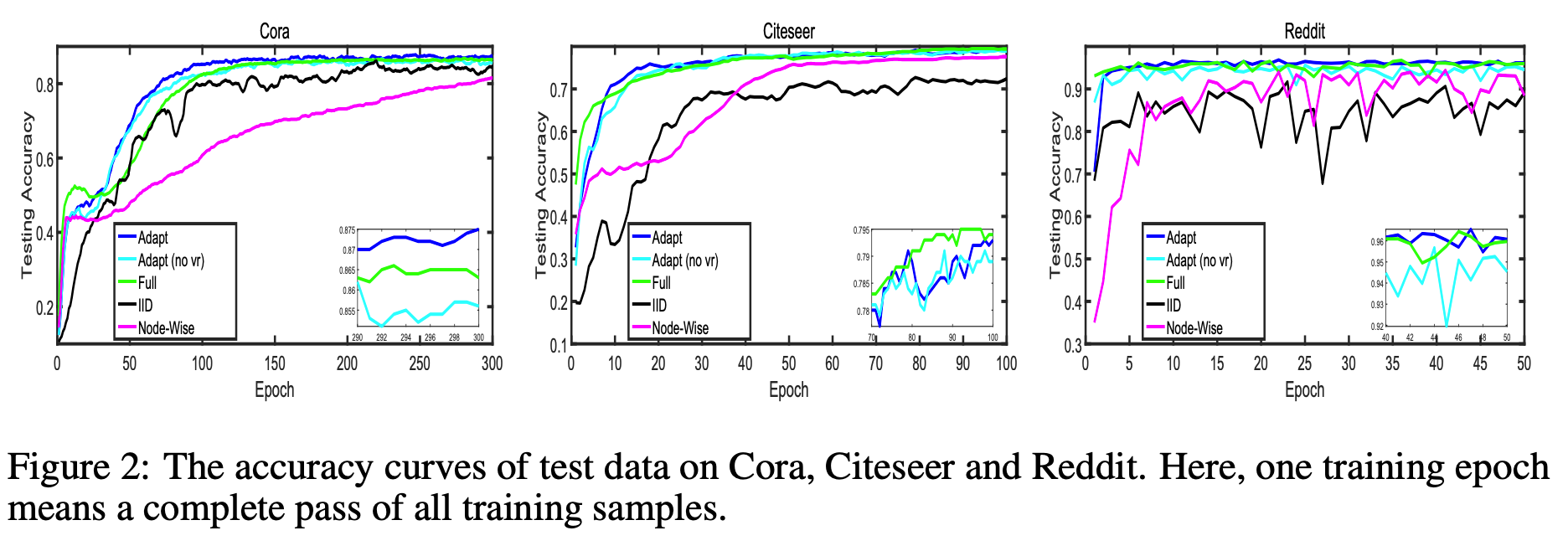
From the learning curves, the performance using layer-wise sampling is comparable to the full training and is better than Node-Wise(re-implementation of GraphSage) and IID(re-implementation of FastGCN). However, the variance reudction seems not to help much here.

Note the leanrning curves above are based on a re-implementation of FastGCN and GraphSage for a fair comparison. The comparison with the official implementation is presented below:

For skip connections, the authors also add a skip connection between the first layer and the last layer. I think skip connection does not help too much on the datasets concerned.