GAT

Summary

Incorporate multi-head attention into GCN, which clearly strengthens its model capacity. The authors claim that this is helpful for inductive learning: where we want to generalize a graph neural network to unseen nodes and graphs.

Attention

The key difference between GAT and GCN is how to aggregate the information from the one-hop neighbourhood.

For GCN, a convolution operation produces the normalized sum of the node features of neighbours.

$$h_i^{(l+1)}=\sigma\left(\sum_{j\in \mathcal{N}(i)} {\frac{1}{c_{ij}} W^{(l)}h^{(l)}_j}\right),$$

where $\mathcal{N}(i)$ is the union of $v_i$ and all its one-hop neighbours, $c_{ij}=\frac{1}{\sqrt{|\mathcal{N}(i)|}}\frac{1}{\sqrt{|\mathcal{N}(j)|}}$ is a normalization constant based on graph structure, $\sigma$ is an activation function such as ReLU, $W^{(l)}$ is a shared weight matrix for node-wise feature transformation.

GAT introduces the attention mechanism as substitute to the statically normalized convolution operation to remove its dependency on graph structure. It aggregates the neighborhood features by assigning different weights to features from neighbor nodes depending on the features of the current node.

$$\begin{align} e_{ij}&=\textbf{LeakyReLU}(\vec a^{T}[Wh_{i}^{(l)}]\|[Wh_{j}^{(l)}]),\\ \alpha_{ij}&=\frac{\exp(e_{ij})}{\sum_{k\in \mathcal{N}(i)}^{}\exp(e_{ik})},\\ h_i^{(l+1)}&=\sigma\left(\sum_{j\in \mathcal{N}(i)} {\alpha_{ij} W^{(l)} h^{(l)}_j }\right), \end{align}$$

where $\|$ is the concatenation operation, $\sigma(\cdot)$ is some activation function, $h_{i}^{(l)}\in\mathbb{R}^{F}$, $W\in\mathbb{R}^{F'\times F}$, $\vec a^{T}\in\mathbb{R}^{1\times 2F'}$. Both $W$ and $\vec a$ are learnable.

Note that employing attention mechanism allows dealing with directed graphs.

Multi-head Attention

Analogous to multiple channels in ConvNet, GAT introduces multi-head attention to enrich the model capacity. The authors claimed that this is beneficial for stabilizing the learning process of self-attention. Basically we can have multiple "suits" of parameters for computing $\alpha_{ij}$ and $W^{(l)}$ in $h_i^{(l+1)}=\sigma\left(\sum_{j\in \mathcal{N}(i)} {\alpha_{ij} W^{(l)} h^{(l)}_j }\right)$.

Formally this can be done by first performing computation for each head and then aggregate the result from each head with

$$\text{concatenation}: h^{(l+1)}_{i} =\|_{k=1}^{K}\sigma\left(\sum_{j\in \mathcal{N}(i)}\alpha_{ij}^{k}W^{k}h^{(l)}_{j}\right)$$

or

$$\text{average}: h_{i}^{(l+1)}=\sigma\left(\frac{1}{K}\sum_{k=1}^{K}\sum_{j\in\mathcal{N}(i)}\alpha_{ij}^{k}W^{k}h^{(l)}_{j}\right),$$

where $K$ is the number of heads. The authors suggest using concatenation for intermediary layers and average for the final layer.

Experiments

Datasets

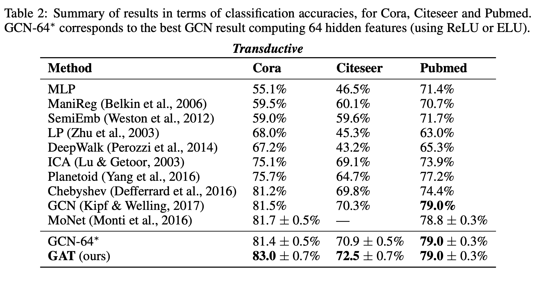
Transductive Learning: They used $3$ standard citation benchmark datasets: Cora, Citeseer and Pubmed. The node features correspond to elements of a bag-of-words representation of a document. Each node has a class label. They allow $20$ nodes per class to be used for training but the training algorithm has access to all of the nodes' feature vectors. The test set consists of $1000$ test nodes and the validation set consists of $500$ nodes.

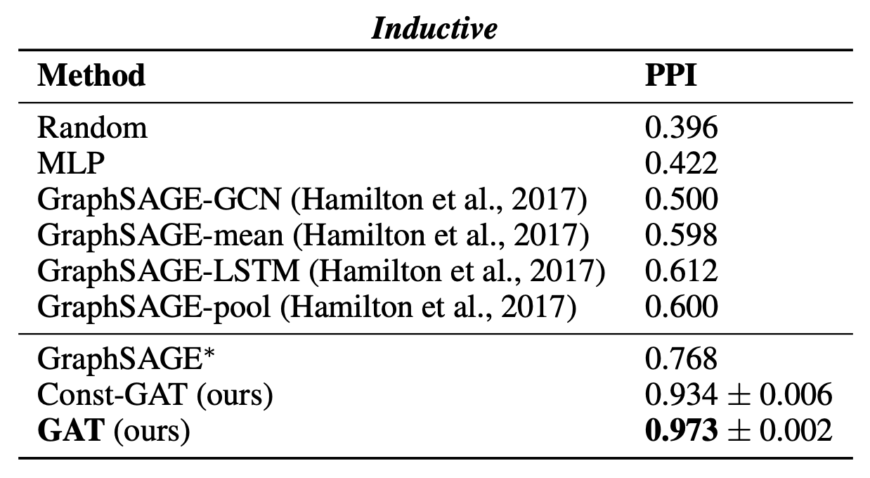
Inductive Learning: They make use of a protein-protein interaction (PPI) dataset that consists of graphs corresponding to different human tissues. For inductive learning, testing graphs remain completely unobserved during training. The node features are composed of positional gene sets, motif gene sets and immunological signatures. There are $121$ labels for each node set from gene ontology, and a node can possess several labels simultaneously.

Below is a summary of dataset statistics:

State-of-the-art Methods

Transductive Learning:

• label propagation

• semi-supervised embedding

• manifold regularization

• skip-gram based graph embeddings

• iterative classification algorithm

• planetoid

• GCN

• ChebyNet

• MoNet

• MLP where no graph structure incorporated

Inductive Learning:

• GraphSAGE-GCN (extends graph convolution to inductive learning): $h_i^{(l+1)}=\sigma\left(\frac{1}{|\mathcal{N}(i)|}\sum_{j\in \mathcal{N}(i)} { W^{(l)} h^{(l)}_j }\right)$

• GraphSAGE-mean (mean pooling)

• GraphSAGE-LSTM

• GraphSAGE-pool (max pooling)

• MLP where no graph structure incorporated

Experimental Setup

Transductive Learning:

• Model: two-layer GAT

• Hyperparameters: optimized based on Cora

• Model flow:

  • $8$ head attention with $F'=8$ features for each head

  • An exponential linear unit (ELU)

  • Classification layer: linear layer with $C$ out features corresponding to $C$ classes, followed by a softmax activation

• Regularization: $L_2$ with $\lambda=0.0005$

• Dropout: $p=0.6$ applied to both layers' inputs as well as to the normalized attention coefficients (at each training iteration, each node is exposed to a stochastically sampled neighborhood).

• For Pubmed, $8$ output attention heads are applied (rather than $1$), with $\lambda=0.001$ for regularization

Inductive Learning:

• Model: three-layer GAT

• Model flow:

  • For the first two layers, $4$ attention heads are used with $F'=256$.

  • An exponential linear unit (ELU)

  • (multi-label) classification layer: $6$ attention heads computing $121$ features each, that are averaged and followed by a logistic sigmoid activation

• Dataset is large enough so no dropout or regularization is required

• Skip connections across the intermediate attention layer

• Batch size $2$ during training

Both models use:

• Glorot (Xavier) initialization

• cross-entropy objective

• Adam with initial learning rate of $0.01$ for Pubmed and $0.005$ for all other datasets

• Early stopping on both the cross-entropy loss and accuracy (transductive) or micro-$F_1$ (inductive) score on the validation nodes, with a patience of $100$ epochs

For the transductive tasks, they report the mean accuracy (with standard deviation) on the test nodes after $100$ runs. For the Chebyshev filter-based approach, they provide the maximum reported performance for filters of orders $K=2$ and $K=3$. For a fair comparison, they further evaluate a GCN model that computes $64$ hidden features, attempting both the ReLU and ELU activation, and reporting the better result after $100$ runs.

For the inductive task, they reported the micro-averaged $F_1$ score on the nodes of the two unseen test graphs, averaged after $10$ runs. When comparing against GraphSAGE, they retune the hyperparameters and denote that variant by $\text{GraphSAGE}^{\ast}$ They also tried a GAT variant with constant attention ($1$ for each node), denoted by $\text{Const-GAT}$.

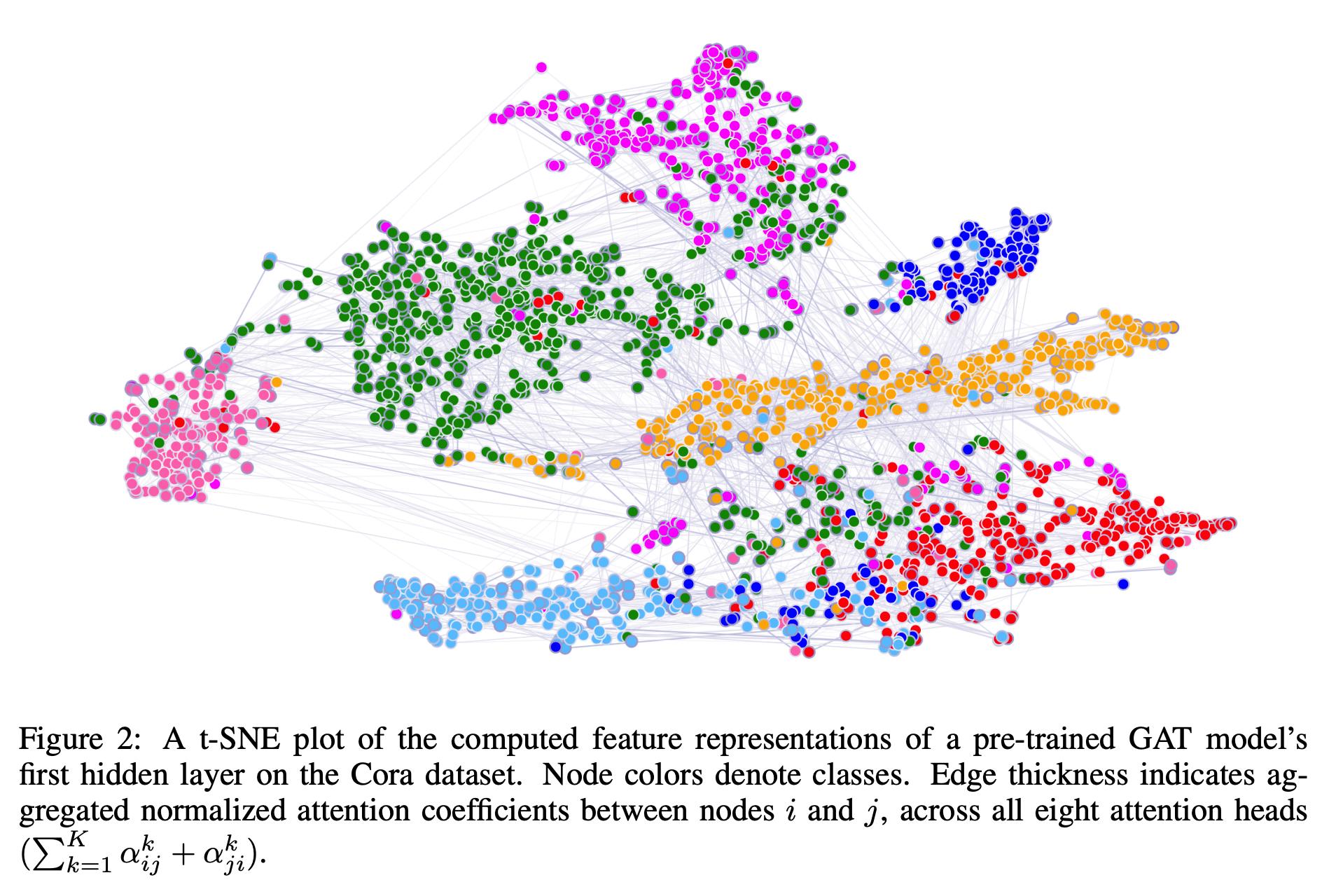
The authors also visualized the representations extracted by the first layer of a GAT pre-trained on the Cora with t-SNE.