Spectral Networks and Deep Locally Connected Networks on Graphs

• Link to paper

Motivation

Generalize ConvNet to graphs.

Spatial Construction

Consider an undirected weighted graph denoted by $G=(V, W)$ where $V=\{1,\cdots, |V|\}$ and $W\in\mathbb{R}^{|V|\times|V|}$ is a symmetric nonnegative matrix.

Locality via W

The weights in a graph determine a notion of locality like the one in images, audio and text. We can restrict attention to sparse "filters" with receptive fields given by neighborhoods, thus reducing the number of parameters in a filter to $O(S\cdot n)$ where $S$ is the average neighborhood size and $n$ is the input feature size.

Multiresolution Analysis in Graphs

The authors mentioned that "[f]inding multiscale clusterings that are provably guaranteed to behave well w.r.t. Laplacian on the graph is still an open area of research" (the publication was in 2014).

Deep Locally Connected Networks

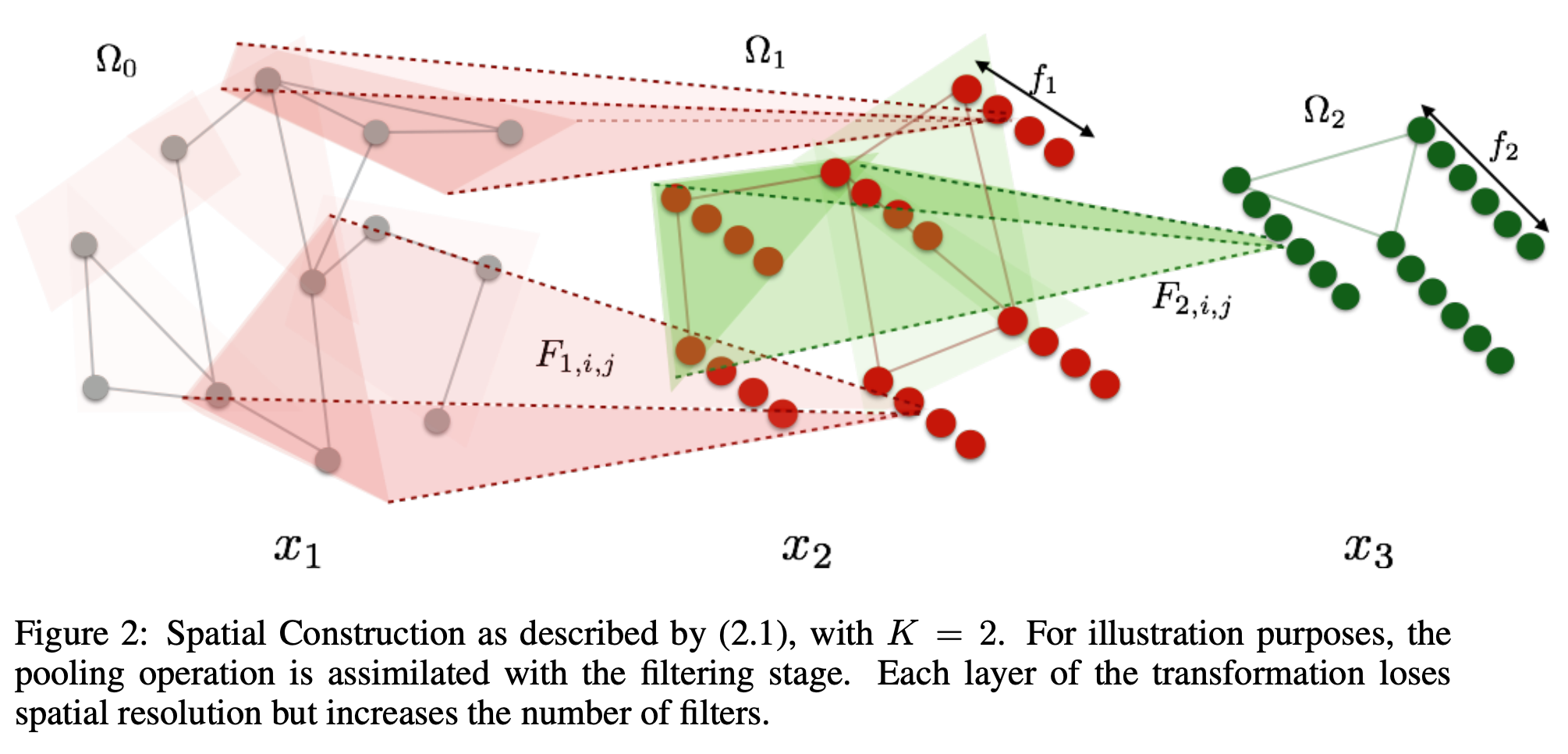
The spatial construction starts with a multiscale clustering of the graph. We consider $K$ scales. We set $V_{0}=V$, and for each $k=1,\cdots, K$, we define $V_{k}$ a partition of $V_{k-1}$ into $d_k$ clusters; and a collection of neighborhoods around each element of $V_{k-1}$:

$$\begin{equation} \mathcal{N}_{k}=\{\mathcal{N}_{k,i}; i=1,\cdots, d_{k-1}\}. \end{equation}$$

With these in hand, we can now define the $k$-th layer of the network as a mapping: $\mathbb{R}^{d_{k-1}\times f_{k-1}}\rightarrow \mathbb{R}^{d_k\times f_k}$, $x_{k}\mapsto x_{k+1}$ defined as

$$\begin{equation} x_{k+1, j}=L_{k}h\left(\sum_{i=1}^{f_{k}-1}F_{k,i,j}x_{k, i}\right), \end{equation}$$

where:

• $x_{k+1,j}$ is the $j$ th column of $x_{k+1}$ and $x_{k, i}$ is the $i$ th column of $x_k$
• $F_{k, i, j}$ is a $d_{k-1}\times d_{k-1}$ sparse matrix with nonzero entries in the locations given by $\mathcal{N}_{k}$
• $L_k$ outputs the result of a pooling operation over each cluster in $V_k$.

This construction is illustrated below:

Started with $W_0=W$, for all $k\leq K$, $V_k$ is constructed by merging all nodes whose pairwise distance (determined by the corresponding entry in $W_{k-1}$) are less than $\varepsilon$. $W_k$ and $\mathcal{N}_{k}$ are then obtained with

$$\begin{align} A_{k}(i, j)&=\sum_{s\in V_k(i)}\sum_{t\in V_{k}(j)}W_{k-1}(s, t),\\ W_{k}&=\text{rownormalize}(A_k),\\ \mathcal{N}_{k}&=\text{supp}(W_k),\\ \end{align}$$

where $V_{k}(i)$ is the $i$ th node in $V_k$, $\text{supp}(W_k)$ is the support of $W_k$, i.e. $\{(i,j):W_k(i,j)>0\}$.

Spectral Construction

The global structure of the graph can be exploited with the spectrum of its graph-Laplacian to generalize the convolution operator.

Harmonic Analysis on Weighted Graphs

The frequency and smoothness relative to $W$ are interrelated through the combinatorial Laplacian $L=D-W$ or graph Laplacian $\mathcal{L}=I-D^{-\frac{1}{2}}WD^{-\frac{1}{2}}$. For simplicity, the authors simply use the combinatorial Laplacian.

If $x$ is an $m$-dimensional vector, a natural definition of the smoothness functional $||\nabla x||_{W}^{2}$ at a node $i$ is

$$\begin{align} ||\nabla x||_{W}^{2}(i)&=\sum_{j}W_{ij}\left(x(i)-x(j)\right)^2,\\ ||\nabla x||_{W}^{2}&=\sum_{i}\sum_{j}W_{ij}\left(x(i)-x(j)\right)^2=2x^{T}\Delta x, \end{align}$$

This definition is also known as the Dirichlet energy. With this definition, the smoothest vector is a constant:

$$\begin{equation} \phi_0=\text{argmin}_{x\in\mathbb{R}^{m}, ||x||=1} ||\nabla x||_{W}^{2}=\frac{1}{\sqrt{m}}\textbf{1}_{m}. \end{equation}$$

Note here $\phi_0$ is also the eigenvector of $L$ corresponding to eigenvalue $0$.

Each successive

$$\begin{equation} \phi_i = \text{argmin}_{x\in\mathbb{R}^{m}, ||x||=1, x\perp\{v_0,\cdots,v_{i-1}\}}||\nabla x||_{W}^{2} \end{equation}$$

is an eigenvalue of $L$, and the eigenvalues $\lambda_i$ allow the smoothness of a vector $x$ to be read off from the coefficients of $x$ in $[\phi_0,\cdots, \phi_{m-1}]$, equivalently as the Fourier coefficients of a signal defined in a grid. The filters are therefore multipliers on the eigenvalues of $\Delta$ and reduces the number of parameters of a filter from $m^2$ to $m$.

Two related results are: 1. Functions that are smooth relative to the grid metric have coefficients with quick decay in the basis of eigenvectors of $\Delta$. 2. The eigenvectors of the subsampled Laplacian are the low frequency eigenvectors of $\Delta$.

Extending Convolutions via the Laplacian Spectrum

Theoretical Formulation

Given two functions $f,g:\Omega\rightarrow\mathbb{R}$, $\Omega$ a Euclidean domain, the convolution of $f$ and $g$ is defined to be

$$\begin{equation} (f\star g)(t)=\int_{\Omega}f(s)g(t-s)ds, \end{equation}$$

where $\int_{\Omega}|f(s)g(t-s)|ds<\infty$.

A famous result related to convolution is the convolution theorem: $\widehat{f\star g}=\hat{f}\cdot\hat{g}$, where $\hat{}$ denotes the fourier transform of a function and $\cdot$ denotes the elementwise multiplication.

The fourier transform of $f\in L^{1}(\mathbb{R})$ is defined by

$$\hat{f}(x)=\int_{\mathbb{R}}f(y)e^{-ixy}dy$$

The description above is for the Euclidean case. To generalize the notion of convolution to non-Euclidean case, one possibility is by using the convolution theorem as a definition.

Since $\Delta$ admits on a compact domain an eigendecomposition with a discrete set of orthonormal eigenfunctions $\phi_0,\phi_1,\cdots$ and they are the smoothest functions in the sense of the Dirichlet energy, they can be interpreted as a generalization of the standard Fourier basis.

We can then define the convolution of $f$ and $g$ on a graph as

$$(f\star g)(x)=\sum_{i\geq 0} \langle f, \phi_i\rangle_{L^{2}(\mathcal{X})}\langle g, \phi_i\rangle_{L^{2}(\mathcal{X})}\phi_i(x),$$

where $\mathcal{X}$ is a graph.

For two vectors $\textbf{f}=(f_1,\cdots, f_n)^{T}$ and $\textbf{g}=(g_1,\cdots, g_n)^{T}$, the convolution of $\textbf{f}$ and $\textbf{g}$ can be calculated by

$$\begin{align} f \star g&= \begin{bmatrix} g_{n} & g_{n-1} & \cdots & g_{1}\\ g_{1} & g_{n} & \cdots & g_{n-1}\\ \vdots & \vdots & \ddots & \vdots\\ g_{n-1} & g_{n-2} & \cdots & g_{n}\\ \end{bmatrix} \begin{bmatrix} f_1\\ \vdots\\ f_n \end{bmatrix}\\ &=\Phi(\Phi^{T}g)\circ(\Phi^{T}f)\\ &=\Phi\text{diag}(\hat{g}_1,\cdots, \hat{g}_n)\Phi^{T}f, \end{align}$$

where $\Phi=(\phi_1,\cdots, \phi_n)$. Note that this formulation depends on the choice of $\Phi$.

Practice

Let $\Phi$ be the eigenvectors of $L$, ordered by eigenvalue. A convolutional layer transforming node features with $\mathbb{R}^{|\Omega|\times f_{k-1}}\rightarrow\mathbb{R}^{|\Omega|\times f_{k}}$, $x_{k}\mapsto x_{k+1}$ can be defined as

$$x_{k+1, j}=h\left(\sum_{i=1}^{f_{k-1}}\Phi F_{k,i,j}\Phi^{T}x_{k, i}\right)=h\left(\Phi \sum_{i=1}^{f_{k-1}} F_{k,i,j}\Phi^{T}x_{k, i}\right), j=1,\cdots, f_k,$$

where $F_{k,i,j}$ is a diagonal matrix and $h$ is a real-valued nonlinearity. Note with our previous theory the update rule corresponds to $f_{k}\times f_{k-1}$ filters and $f_{k}\times f_{k-1}\times |\Omega|$ parameters.

Often only the first $d$ eigenvectors of the Laplacian are useful, which carry the smooth geometry of the graph. We can treat $d$ as a hyperparameter and replace $\Phi$ by $\Phi_d$ in the equation above, which only keeps the first $d$ columns of $\Phi$.

This construction can suffer when the individual high frequency eigenvectors are not meaningful but a cohort of high frequency eigenvectors contain meaningful information. It is also not obvious how to do either the forwardprop or the backprop efficiently while applying the nonlinearity on the space side.

The construction above requires $O(|\Omega|)$ parameters. One possibility to use $O(1)$ parameters instead is to employ

$$\text{diag}(F_{k,i,j})=\mathcal{K}\alpha_{k,i,j},$$

where $\mathcal{K}$ is a $d\times q_k$ fixed qubic spline kernel and $\alpha_{k,i,j}$ spline coefficients. The theory for this part seems to be ambiguous.